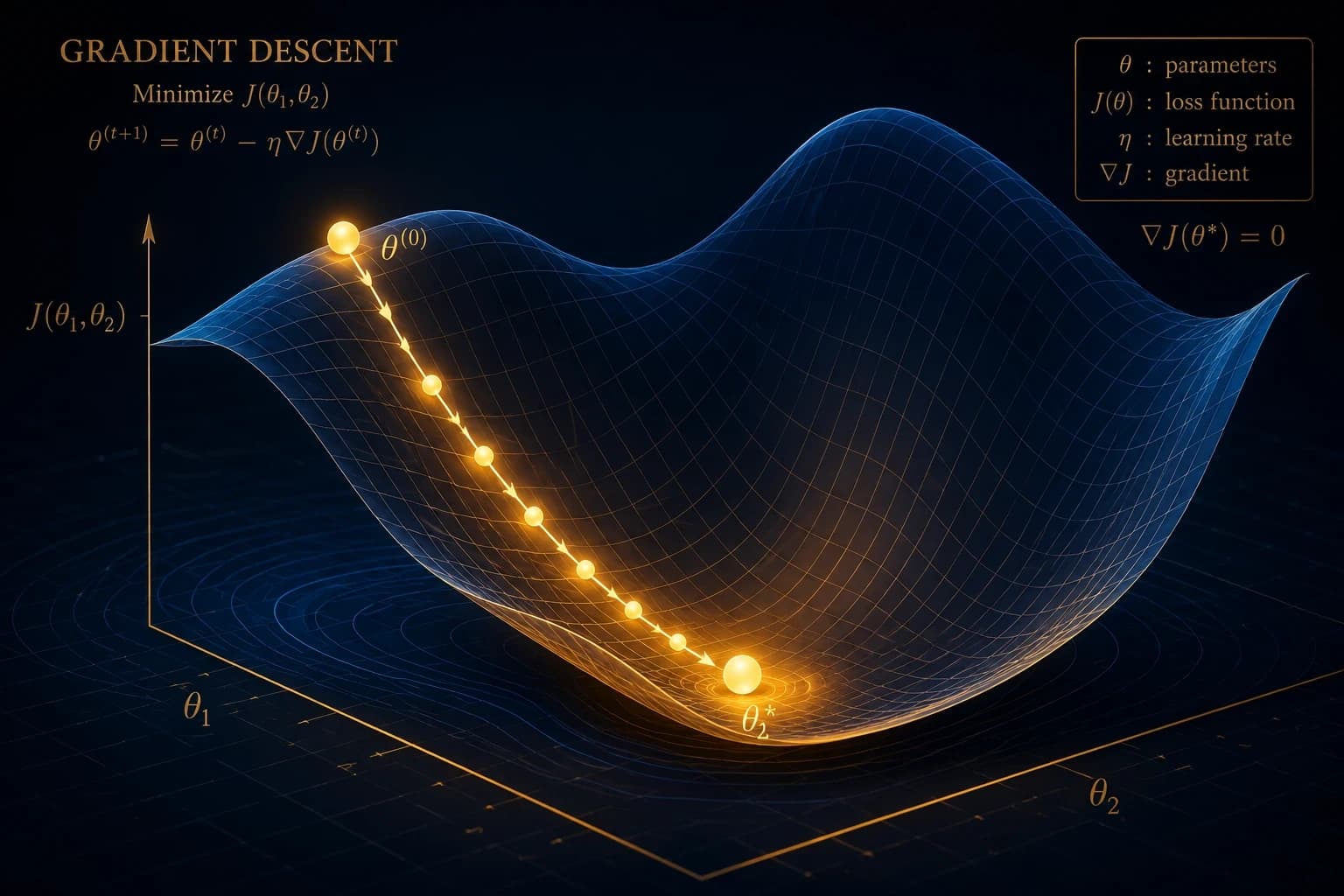
The Journey to AI Part 2 - How a Machine Learns

The Journey to AI Part 2

How a Machine Learns: The Guess→Check→Adjust Loop That Changed Everything

From one artificial neuron to AlexNet, the mechanics that make modern AI possible.

Part 2 of 4 in “The Journey to AI Agents”

Here’s the question nobody asks out loud: when we say a machine “learned” something, what actually happened?

Not the philosophy. The mechanics. What literally happened inside?

Because once you see it, you’ll realize the entire deep-learning revolution from a 1957 artificial neuron to GPT-4 runs on the same four-step loop. Billions of parameters, trillion-token datasets, million-dollar GPUs. Same loop.

Let’s build it from scratch.

Learning Is Just Finding a Function

At its core, any intelligent behavior is a function:

input → [some transformation] → output

Image in → “cat” or “not cat.” Hours studied → exam score. English sentence → French translation.

The difference between Symbolic AI and Machine Learning is who writes that transformation:

• Symbolic AI: a human writes it (as if-then rules)
• Machine Learning: the machine finds it from examples

And “finding” it is surprisingly mechanical. You start with a function of a fixed shape but with adjustable knobs inside. “Learning” means turning those knobs until the function gives correct answers.

These knobs are called parameters or weights.

When you hear “GPT-4 has hundreds of billions of parameters”, that’s billions of these knobs.

The Loop: Guess → Check → Adjust

Make it concrete. Predict exam score from hours studied:

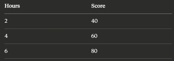
Your function with one knob w: score = w × hours

1. Guess. Try w = 5. For 2 hours, predicts 10. Real answer: 40. Off by 30.
2. Check the error. This “how wrong am I” number is the loss. Goal: make it small.
3. Adjust. Too low → nudge w up. Try w = 8. Better. Nudge again.
4. Repeat thousands of times, nudging in whatever direction shrinks the loss.

Best fit lands around w ≈ 13.6 close across all rows, perfect for none. That's realistic: real data is messy; the machine finds the knob with the smallest error across all examples, not a magic perfect fit.

Two things just happened that matter enormously:

Nobody told the machine the rule. It discovered the relationship by minimizing error.

It generalizes. Ask about 5 hours (never in the training data) → it answers ≈68. It learned the pattern, not just the rows. This is how ML escapes the brittleness that killed Symbolic AI.

The Perceptron: An Artificial Neuron (1957)

With the goal clear, Frank Rosenblatt took inspiration from the human brain to find functions from examples.

A real brain neuron receives signals from other neurons and “fires” if the combined signal crosses a threshold; otherwise it stays quiet. Rosenblatt built an artificial version: the perceptron.

input x1 ──(weight w1)──┐
                        ├──►  sum = w1·x1 + w2·x2  ──►  if sum > threshold: 1 (fire)
input x2 ──(weight w2)──┘                                                   0 (quiet)

Each weight means: “how much does this input matter?” It learns the weights via the same guess→check→adjust loop above.

The New York Times reported that the Navy expected this machine to “walk, talk, see, write, and reproduce itself.”

Real hype. From a math paper about a single neuron.

The Wall: XOR

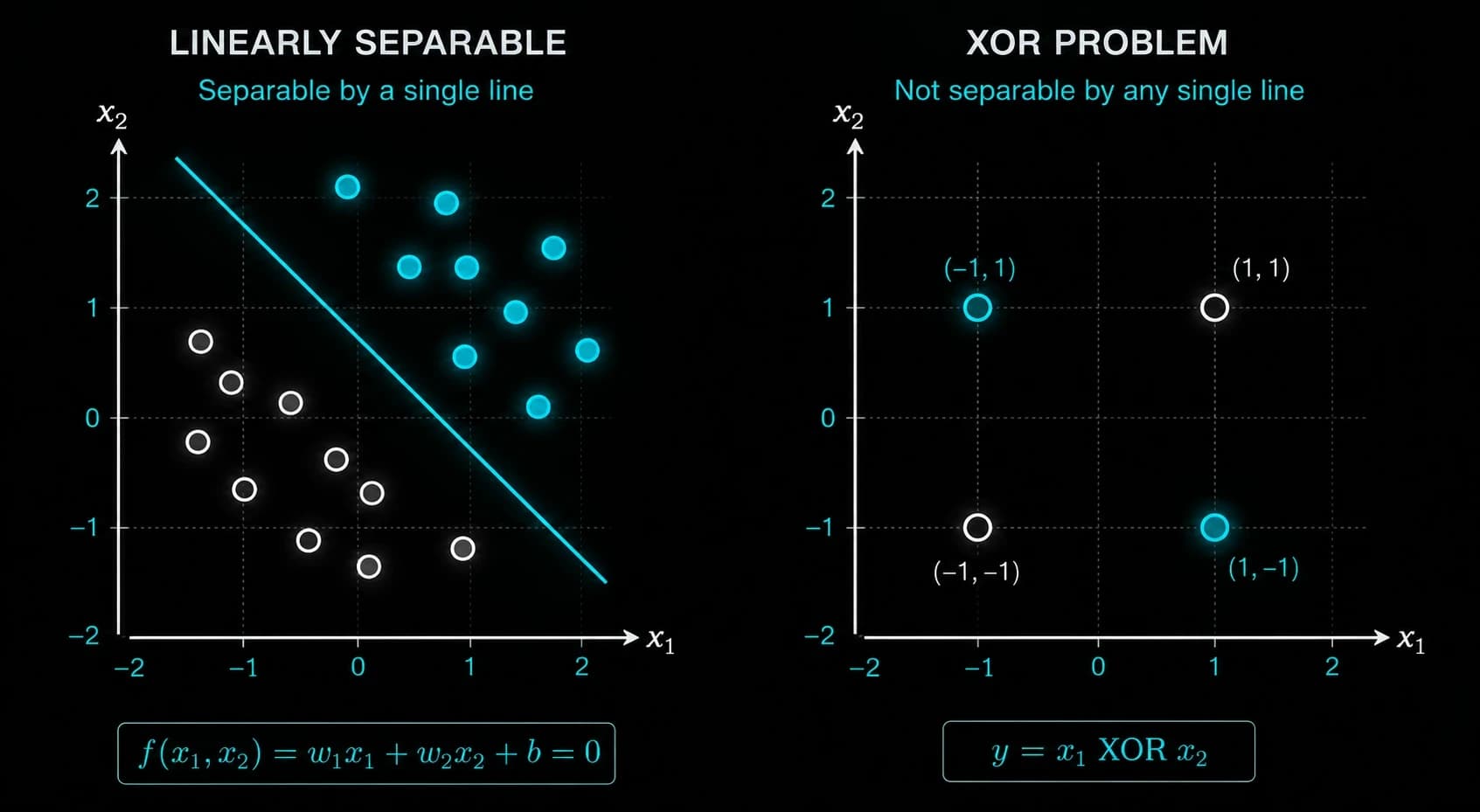
Geometrically, a perceptron draws one straight line to separate “fire” from “don’t fire.”

For some problems, like AND, one line is enough. For XOR (fire if the inputs are different), it isn’t:

XOR:

x2
   1  |  ●        ○
      |
   0  |  ○        ●
      +──────────────  x1
         0        1

The ● points are diagonal. No single straight line can separate them from ○.
It's geometrically impossible.

In 1969, Minsky and Papert proved this formally. Neural-net research lost funding for over a decade. The “connectionist winter.”

The fix was obvious: stack neurons in layers. A first layer bends the problem space; a second layer draws its line in the bent space, and XOR becomes solvable. But stacking raised a brutal new question:

How do you train the hidden layers?

The output layer has a target to compare against. The neurons in the middle don’t. Nobody told them what they were supposed to output. Nobody knew how to tune their knobs.

That question froze the field.

Backpropagation: Blame Flows Backward (1986)

Rumelhart, Hinton, and Williams answered the question in 1986. It’s called backpropagation, and it’s still how every neural network trains today.

The key insight: a neural network is just functions stuffed inside functions.

output = layer3( layer2( layer1( input ) ) )

The loss (error) sits at the output. Any buried weight affects the loss through a chain of steps. Calculus’s chain rule says: the total sensitivity of a buried weight on the loss equals the product of all the local sensitivities along the chain.

Think of it as a corporate org chart:

The company ships a bad product (high loss). The CEO knows the result is off by X. She tells each VP exactly how much they contributed. Each VP adjusts their own work and tells their managers how far off they were. Blame flows backward down the hierarchy. Each level owns its slice and passes the rest along.

By the end, every employee (weight) knows exactly how to adjust, including those buried deep in the org chart. Nobody needed a “correct answer” for the middle layers; the blame distributed itself backward from the single known error at the top.

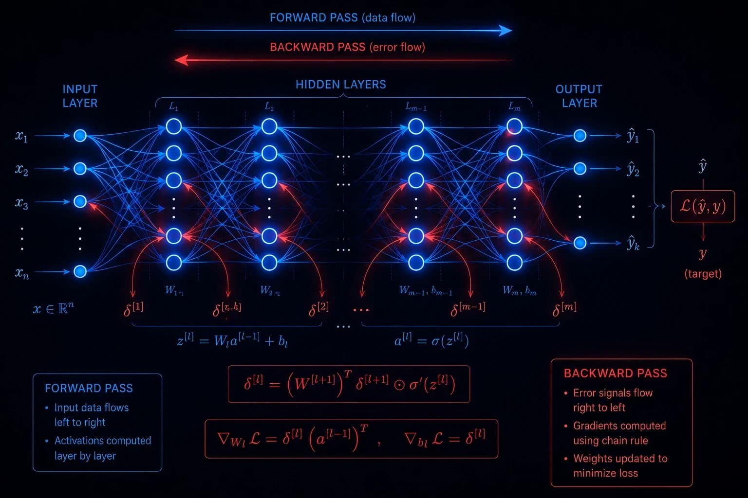
In practice, it’s two passes:

1. Forward pass: feed input through, compute the prediction and loss. “How wrong are we?”
2. Backward pass: start at the loss, push the error backward layer by layer. Each layer calculates its own gradient (which direction to nudge) and passes the signal further back.

Then nudge every weight one small step in its error-reducing direction. Repeat millions of times.

Hidden layers could finally learn. Stacked networks could finally train. The winter was over.

Deep Learning: Why It Took Another 25 Years

Backprop worked in 1986. Yet deep learning didn’t change the world until 2012. Three walls had to fall first.

Wall 1 — Not enough data.

A deep network has millions of knobs. With only a few thousand examples, it doesn’t learn the pattern. It memorizes the training set (called overfitting) and fails on anything new. Lots of knobs demand lots of data.

Wall 2 — Not enough compute.

Training means running millions of examples through millions of weights, forward and backward, millions of times. On 1990s CPUs, training a serious deep net could take months. Nobody iterates on month-long experiments.

Wall 3 — Vanishing gradients.

The chain rule multiplies local sensitivity values along the chain. Old activation functions (like sigmoid) squashed their outputs to small numbers. Multiply small numbers through many layers:

0.2 × 0.2 × 0.2 × 0.2 × 0.2 ≈ 0.0003

The error signal vanished before reaching the early layers. The foundational layers, the ones learning basic features everything else builds on, barely got any learning signal. Deep networks were, in practice, untrainable past a few layers.

All Three Walls Fall at Once (~2006–2012)

Data arrived. The internet produced massive labeled datasets. The landmark: ImageNet 14 million hand-labeled images across 1,000 categories. Suddenly, millions of knobs had enough examples to generalize.

GPUs arrived. A GPU was built to render video games: run the same simple math on thousands of numbers simultaneously. It turns out a neural network’s core operation is exactly that matrix multiplication, repeated across entire layers. Researchers repurposed gaming hardware and got 10–100× faster training. Months became days.

Training tricks arrived. The key one: ReLU activation. Its local rate is just 1 for active neurons. Multiply 1 × 1 × 1 × 1 all the way back, and the gradient doesn’t vanish. Early layers were finally learned.

AlexNet (2012): The Watershed

The proof arrived at the ImageNet Large Scale Visual Recognition Challenge in 2012.

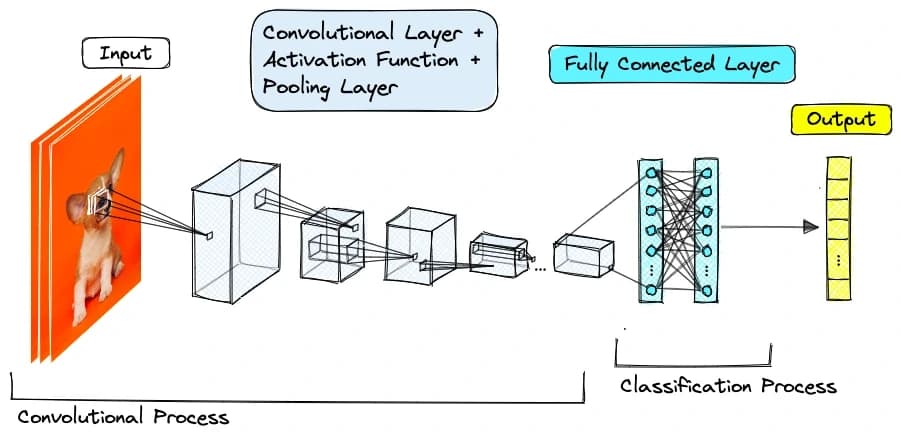
A deep network called AlexNet (Krizhevsky, Sutskever, Hinton) many layers, trained on GPUs, didn’t just win. It demolished every hand-engineered approach by a massive margin.

The result flipped the field overnight. Everyone saw: depth works now, given the right data and compute. The modern AI era starts here.

And notice what it proved about the old obstacle from Part 1 — Crack #4: Perception is inarticulate. Nobody wrote rules for recognizing cars or cats. The network discovered its own features by stacking layers:

raw pixels
  → layer 1: edges and color blobs
    → layer 2: corners, curves, textures
      → layer 3: eyes, wheels, ears
        → layer 4: "this arrangement of parts = cat"

Symbolic AI’s hardest unsolved problem perception fell to three ingredients working together:

Depth      → learns hierarchical features (no hand-engineering)
+ Big Data   → millions of examples, knobs generalize instead of memorize
+ GPUs       → training finishes this decade, not the next
= Deep Learning

Pull any one out, it collapses. All three together, and it changes the world.

What’s Next

We can now build networks that see and recognize. But language is a different beast entirely. Before a network can read a sentence, someone has to solve a problem that sounds almost trivial:

How do you hand the word “king” to a machine that can only multiply numbers?

The answer is one of the most beautiful ideas in all of machine learning.

Part 3: “Teaching Machines to Read - How Words Became Coordinates”

Tags: Deep Learning, Neural Networks, Backpropagation, Machine Learning, AI History

Originally published on Medium on June 25, 2026.